PyTorch Learning Series: Part 3

Hey Everyone! 👋 Welcome to the Part:3 of the pytorch learning series.

I hope you liked the Part:2 of this series and have gotten a pretty good idea about Tensors in PyTorch.

If you haven’t read the Part:1 and Part:2 yet, I would recommend stopping here, finishing them first and then resuming this part.

Moving forward in the series, in this blog we will be learning about a super-important concept in PyTorch called “Autograd”.

Here’s the agenda of this blog:

1. Understanding differentiation and its complexity
2. Why Autograd?
3. What is Autograd? (A detailed walkthrough with hands-on coding)
4. How to disable Gradient Tracking?

Now that we have a clear plan in mind, let’s get right into this super interesting and powerful topic and dismantle it from the very basics.

The very first question that tickled my mind listening to this term: “Autograd” was that, is it something related to differentiation? Well if the same has hit your mind as well, then yes you are right. It is heavily coupled with gradient or in simple terms differentiation.

Then why not use simple differentiation which we have learnt in our high-school mathematics? You are not wrong in raising this question. But in terms of neural networks and complex architectures, it is not that simple. Let’s understand why and I assure you that you surely will appreciate Autograd.

Differentiation and its complexity

So when talking about differentiation, here I am not talking about about us who will do it on pen and paper. It is to be performed by the computers during training neural networks and doing the same with code is not as simple as it sounds.

Let’s take some examples and try to manually code the differentiation function.

Example 1:

So in order to calculate the gradient for any x, we can write the differentiation function as

def dy_dx(x):
	return 2*x

If we want to calculate the gradient of y at x=2, we can just call the function dy_dx(2) and we will get our desired result.

Example 2:

The differentiation function becomes

import math

def dy_dx(x):
	return 2*x*math.cos(x**2)

As you can observe, the differentiation function became more complex than the function in Example 1. The reason is the chained functions.

In the first example, the gradient we needed involved a direct dependency, where y was dependent directly on x. But in the 2nd example, we wanted gradient of z w.r.t x, but z was not directly dependent on x. z was a function of y, and y was a function of x. Hence we needed to apply chain rule of differentiation to compute the gradient.

Example 3:

import math
def dy_dx(x):
	return 2 * x * math.cos(x**2) * math.exp(math.sin(x**2))

As you can clearly see, this function has become much more complex than the previous examples we saw. And this keeps getting complex when we have more chained and dependent functions.

Hence, it is humanly impossible to keep writing such gradients manually for more complex real-world functions. This is why Autograd came into existence and it makes our life easier. Let’s now understand why autograd is important in context of deep learning and neural networks!

Why is Autograd important?

Now that we have built an intuition around differentiation and chain rule, this is the perfect moment to connect everything to how a neural network actually learns.

Let’s take a very simple neural network and understand what is happening step by step.

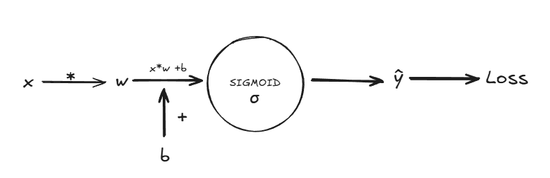
The diagram above might look intimidating at first, but trust me — once we break it down, it will feel extremely logical.

The Problem Setup

We are given a dataset that looks something like this:

• Input (x): CGPA
• Output (y): Whether the student got placed (1 = Yes, 0 = No)

So essentially, we want our model to answer this question:

Given a CGPA, what is the probability that the student gets placed?

This is a binary classification problem, and for such problems, the Sigmoid function is a natural choice.

Step 1: Forward Pass (Making a Prediction)

This is where everything starts.

Linear Transformation

The first operation the model performs is a simple linear equation:

$z = w*x + b$

Here:

• x → input (CGPA)
• w → weight (learnable parameter)
• b → bias (learnable parameter)

At this stage, the model is just doing basic math — no learning yet.

Activation Function (Sigmoid)

The output z is then passed through the Sigmoid function:

$ŷ = σ(z) = 1/1+ e^-z$

So now:

• ŷ ≈ 1 → high chance of placement
• ŷ ≈ 0 → low chance of placement

This ŷ is our model’s prediction.

Step 2: Loss Calculation (How Wrong Are We?)

Prediction alone is not enough.

We need to know how good or bad that prediction is.

For binary classification, we use Binary Cross-Entropy Loss:

Where:

• y → actual label (0 or 1)
• ŷ → predicted probability

Intuition:

• If the prediction is close to the actual value → loss is small
• If the prediction is very wrong → loss becomes large

Loss is just a number that tells the model:

“Hey, this prediction was this much wrong.”

Step 3: Backward Pass (This Is Where Learning Happens)

Now comes the most important part — learning from mistakes.

The goal is simple:

Adjust w and b such that the loss becomes smaller.

To do this, we compute gradients:

But notice something important here

• The loss depends on ŷ
• ŷ depends on z
• z depends on w and b

This is exactly the same chained dependency we discussed earlier.

So the gradients are computed using the chain rule.

Imagine writing the functions manually for computing these gradients. Would be a nightmare right!

And here is where Autograd shines — it automatically computes all these gradients for us, without requiring us to manually write the functions for these.

Why This Matters

Everything we discussed earlier about:

• differentiation
• chained functions
• complex gradients

…comes together here.

A neural network is nothing but a huge mathematical function, and training it means computing gradients efficiently. Now for a dense complex neural network, imagine how complex these equations will get and manually writing python functions for their gradient is nearly impossible. Autograd helps us to exactly do that.

What is Autograd?

Let’s first see the formal definition of Autograd:

Autograd is a core component of PyTorch that provides automatic differentiation for tensors operations. It enables gradient computations, which is essential for training machine learning models using optimization algorithms like gradient descent.

Well now that we know why autograd is required and what is autograd (well just the definition till now), as we do in every blog, let’s get our hands dirty and learn autograd the coding way!

import torch

x = torch.tensor(3.0, requires_grad=True)
x

Output

tensor(3., requires_grad=True)

If you observe carefully, in the previous part, whatever tensor we created, it didn't has this requires_grad=True attribute. This is because by default, PyTorch tensors do not track gradients and the value of this parameter is False. But when we want to track gradients, we need to explicitly set requires_grad=True. And in this case we want to track gradients for x, i.e, we want to calculate the derivative of this tensor, and hence we set requires_grad=True. What this does is it allows PyTorch to track all operations on this tensor from now on, and whenever we need the derivative w.r.t this tensor, PyTorch will be able to compute it.

Whenever we would need derivative of a tensor, during creation of that tensor make the requires_grad parameter as True.

Now let's create a relationship with this tensor.

y = x**2

y

Output

tensor(9., grad_fn=<PowBackward0>)

There is a new param returned called grad_fn which is the function that computed this tensor. This is the gradient function. So it tells PyTorch that how y is related to x.

What happens internally is that, PyTorch creates a computation graph. It is a directed acyclic graph (DAG) that represents the sequence of operations that were performed to compute the output.

In this case the graph would look something like this.

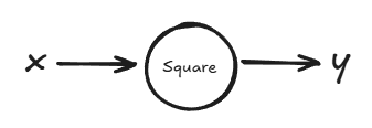
Now when we move from left to right in this computation graph, we are using x to caclculate y. But if we move from right to left, we are using y to calculate x, which means we are calculating dy/dx

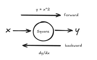
Now to calculate this dy/dx, we use the backward() method.

y.backward()

As soon as we call this method, PyTorch will compute the gradient of y w.r.t x and store it in x.grad.

x.grad

Output:

tensor(6.)

Even if it is a more complex computation graph, calling the backward() method will compute the gradient of the output w.r.t the input for which we have enabled gradient tracking.

Example 2:

Let's use the 2nd example we saw above, and try to find the derivative using autograd.

The manual function to calculate this would be:

import math

def dz_dx(x):
    return 2 * x * math.cos(x**2)

dz_dx(4)

Output:

-7.661275842587077

Now let's do the same using Autograd

x = torch.tensor(4.0, requires_grad=True)

y = x ** 2

z = torch.sin(y)

Now we have defined our functions and let's print and see them.

x
y
z

Output:

tensor(4., requires_grad=True)
tensor(16., grad_fn=<PowBackward0>)
tensor(-0.2879, grad_fn=<SinBackward0>)

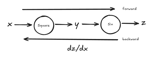
Now let's calculate the gradient.

z.backward()

x.grad

Output:

-7.661275842587077

And as you can see, it is the exact same value which we got when we calculated this gradient using manual python function.

A question that came to my mind, and it might have crossed yours too is that, to calculate gradient of z w.r.t x we also need to calculate gradient of y w.r.t x and then multiply it with gradient of z w.r.t y, that is we need intermediate gradients.

So let's try accessing an intermediate gradient.

y.grad

Output:

<ipython-input-59-10b3a7061f6d>:1: UserWarning: The .grad attribute of a Tensor that is not a leaf Tensor is being accessed. Its .grad attribute won't be populated during autograd.backward(). If you indeed want the .grad field to be populated for a non-leaf Tensor, use .retain_grad() on the non-leaf Tensor. If you access the non-leaf Tensor by mistake, make sure you access the leaf Tensor instead. See github.com/pytorch/pytorch/pull/30531 for more informations. (Triggered internally at aten/src/ATen/core/TensorBody.h:489.)
  y.grad

As you can see, it throws an Error. This is because y is not a leaf tensor, it is a result of some operation on x. Internally we can only access the gradients of leaf tensors. So in our example, we started from z and were going backward till x. Hence z is the root tensor and x is the leaf tensor.

The intermediate tensors gradient are calculated but not accessible to us as we didn't explicitly mentioned that we would need it later.

But we can also access, them by using retain_grad() method. When creating the intermediate tensor for which we would like to access the gradient, we call retain_grad() with it which tells PyTorch to make the gradients of that tensor accessible to us after the backfward pass.

y = x**2
y.retain_grad()

After creating y, we call retain_grad() on it.Now after the z.backward(), if we call y.grad it will be accessible.

y.grad

Output:

tensor(-0.9577)

If you are curious to know more about this, you can read it here: Leaf vs Non-Leaf

Now let's try and see autograd in action for a Neural Network which will clear the concept of autograd in a better way.

Example 3: Neural Network

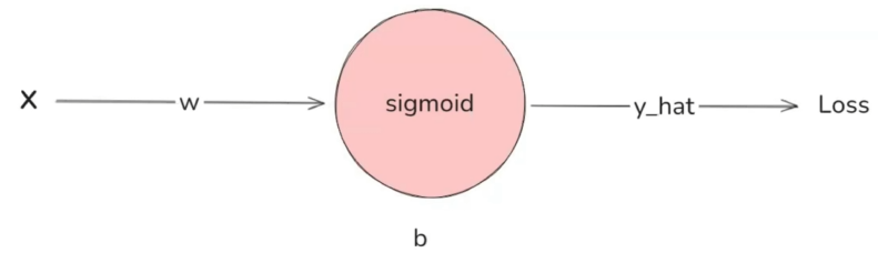
1. Linear Transformation

1. Activation (Sigmoid Function):

1. Loss Function (Binary Cross-Entropy Loss):

Now in this neural network we will need to calculate 2 derivatives

Derivative of Loss wrt w = $\frac{dL}{dw}$

Derivative of Loss wrt z = $\frac{dL}{dz}$

Now if we write the mathematical equations for calculating these derivatives, they will be:

Now let's code the derivatives manually first

import torch

# Inputs
x = torch.tensor(6.7) # Input feature
y = torch.tensor(0.0) # True label (binary)

# Parameters
w = torch.tensor(1.0) # Weight
b = torch.tensor(0.0) # Bias

We start by defining our input x (CGPA = 6.7) and the true label y (0 = not placed). We also initialize our weight w and bias b with some starting random values.

# Binary Cross-Entropy Loss for scalar
def binary_cross_entropy_loss(prediction, target):
    epsilon = 1e-8  # To prevent log(0)
    prediction = torch.clamp(prediction, epsilon, 1 - epsilon)
    return -(target * torch.log(prediction) + (1 - target) * torch.log(1 - prediction))

This is our loss function. The epsilon is a small value to prevent taking log of 0, which would give us infinity. The clamp function ensures our prediction stays within valid bounds.

# Forward pass
z = w * x + b  # Weighted sum (linear part)
y_pred = torch.sigmoid(z)  # Predicted probability

# Compute binary cross-entropy loss
loss = binary_cross_entropy_loss(y_pred, y)

Here we perform the forward pass — first computing the linear transformation z, then passing it through sigmoid to get a probability, and finally computing the loss.

loss

Output

tensor(6.7012)

Our loss is around 6.7 which is quite high. This makes sense because with w=1 and b=0, our model predicts a high probability of placement for CGPA 6.7, but the actual label is 0 (not placed). The model is very wrong!

Now comes the tedious part — manually computing the gradients using chain rule.

# Derivatives:
# 1. dL/d(y_pred): Loss with respect to the prediction (y_pred)
dloss_dy_pred = (y_pred - y)/(y_pred*(1-y_pred))

# 2. dy_pred/dz: Prediction (y_pred) with respect to z (sigmoid derivative)
dy_pred_dz = y_pred * (1 - y_pred)

# 3. dz/dw and dz/db: z with respect to w and b
dz_dw = x  # dz/dw = x
dz_db = 1  # dz/db = 1 (bias contributes directly to z)

dL_dw = dloss_dy_pred * dy_pred_dz * dz_dw
dL_db = dloss_dy_pred * dy_pred_dz * dz_db

We broke down the chain rule into 3 parts: the derivative of loss w.r.t prediction, the derivative of sigmoid, and the derivative of the linear transformation. Then we multiplied them all together.

print(f"Manual Gradient of loss w.r.t weight (dw): {dL_dw}")
print(f"Manual Gradient of loss w.r.t bias (db): {dL_db}")

Output

Manual Gradient of loss w.r.t weight (dw): 6.691762447357178
Manual Gradient of loss w.r.t bias (db): 0.998770534992218

As you can see, we manually applied the chain rule step by step. We calculated each intermediate derivative and then multiplied them together to get the final gradients.

Now let's do the same using Autograd

# Inputs
x = torch.tensor(6.7, requires_grad=True) # Input feature
y = torch.tensor(0.0, requires_grad=True) # True label (binary)

# Parameters
w = torch.tensor(1.0, requires_grad=True) # Weight
b = torch.tensor(0.0, requires_grad=True) # Bias

Notice the key difference here — we added requires_grad=True to our tensors. This tells PyTorch to track all operations on these tensors so it can compute gradients later.

Notice we didn't add requires_grad=True to x and y because we don't need gradients for them.

# Forward pass
z = w * x + b  # Weighted sum (linear part)
z

Output

tensor(6.7000, grad_fn=<AddBackward0>)

y_pred = torch.sigmoid(z)
y_pred

Output

tensor(0.9988, grad_fn=<SigmoidBackward0>)

Our predicted probability is 0.9988, meaning the model thinks there's a 99.88% chance of placement. The grad_fn=<SigmoidBackward0> tells us this came from a sigmoid operation.

loss = binary_cross_entropy_loss(y_pred, y)
loss

Output

tensor(6.7012, grad_fn=<NegBackward0>)

Same loss value as before! The computation graph is now complete — PyTorch has tracked every operation from inputs to loss.

Now here's where the magic happens. One simple call to backward() and PyTorch computes all the gradients for us.

loss.backward()

This single line traverses the entire computation graph backwards and computes all the gradients using the chain rule. No manual math needed!

w.grad
b.grad

Output

tensor(6.6918)
tensor(0.9988)

And there we have it! The gradients are 6.6918 for weight and 0.9988 for bias — matching our manual calculations. We got the same result without writing a single derivative equation. That's the power of autograd!

Example 4: Gradients with Tensor Arrays

So far, we've been working with scalar input tensors. But what happens when we have a tensor with multiple elements? Let's see how autograd handles that.

x = torch.tensor([1.0, 2.0, 3.0], requires_grad=True)
x

Output

tensor([1., 2., 3.], requires_grad=True)

Now let's define a function that takes this tensor and returns a scalar output. This is important because backward() works on scalar outputs by default.

y = (x ** 2).mean()
y

Output

tensor(4.6667, grad_fn=<MeanBackward0>)

Here, we squared each element and then took the mean. Let's break down what's happening:

• $x = [1.0, 2.0, 3.0]$
• $x^2 = [1.0, 4.0, 9.0]$
• $mean(x^2) = (1 + 4 + 9) / 3 = 14/3 ≈ 4.6667$

Now let's compute the gradients.

y.backward()

x.grad

Output

tensor([0.6667, 1.3333, 2.0000])

And look at that — we got 3 gradients, one for each element in our input tensor!

Let's verify this mathematically. If $y = \frac{1}{n} \sum_{i} x_i^2$, then:

For our case with $n = 3$:

• $\frac{\partial y}{\partial x_1} = \frac{2 \times 1}{3} = 0.6667$
• $\frac{\partial y}{\partial x_2} = \frac{2 \times 2}{3} = 1.3333$
• $\frac{\partial y}{\partial x_3} = \frac{2 \times 3}{3} = 2.0$

This matches exactly with what autograd computed! So when you have a tensor with multiple elements, autograd computes the gradient for each element independently, telling you how much each individual element contributes to the final output. This is incredibly useful in neural networks where we have weight matrices with thousands of parameters — each weight gets its own gradient!

Disabling Gradient Tracking

Sometimes, you don't want PyTorch to track gradients. This is common during inference (when you're just making predictions, not training) or when you want to freeze certain parameters. PyTorch gives us 3 ways to disable gradient tracking:

1. requires_grad_(False) — Modify tensor in-place to stop tracking
2. detach() — Create a new tensor without gradient history
3. torch.no_grad() — Context manager to disable tracking for a block of code

Let's explore each one!

Option 1: requires_grad_(False)

This method modifies the tensor in-place to disable gradient tracking.

x = torch.tensor(3.0, requires_grad=True)
x

Output

tensor(3., requires_grad=True)

We created a tensor with gradient tracking enabled. Now let's disable it.

x.requires_grad_(False)
x

Output

tensor(3.)

Notice how requires_grad=True is gone! The tensor no longer tracks gradients. The underscore _ at the end of the method name is a PyTorch convention indicating an in-place operation — the original tensor is modified.

y = x ** 2
y

Output

tensor(9.)

See? No grad_fn attached to y. Since x doesn't track gradients anymore, neither does y.

Option 2: detach()

This method creates a new tensor that shares the same data but is detached from the computation graph.

x = torch.tensor(3.0, requires_grad=True)
z = x.detach()
z

Output

tensor(3.)

z is a copy of x but without any gradient tracking. The key difference from requires_grad_(False) is that the original tensor x is unchanged.

x

Output

tensor(3., requires_grad=True)

x still has gradient tracking! Only z is detached. This is useful when you want to use a tensor's value without affecting the original computation graph.

y = x ** 2
y1 = z ** 2

y

Output

tensor(9., grad_fn=<PowBackward0>)

y1

Output

tensor(9.)

y has a grad_fn because it came from x (which tracks gradients). But y1 has no grad_fn because it came from z (which is detached).

Option 3: torch.no_grad()

This is the most commonly used method, especially during inference. It's a context manager that temporarily disables gradient tracking for all operations inside it.

x = torch.tensor(3.0, requires_grad=True)

with torch.no_grad():
    y = x ** 2
    
y

Output

tensor(9.)

Even though x has requires_grad=True, the operation inside torch.no_grad() doesn't track gradients. This is super efficient because PyTorch doesn't need to build the computation graph.

x

Output

tensor(3., requires_grad=True)

And importantly, x still has gradient tracking enabled! The torch.no_grad() context only affects operations inside the block, not the tensors themselves.

This is the preferred method during inference because:

• It's clean and readable
• It's temporary (doesn't modify your tensors permanently)
• It saves memory by not storing the computation graph

When to Use What?

Summary

In this part of PyTorch Learning Series, we covered:

• Why differentiation is complex — Manual gradient computation becomes a nightmare as functions get chained
• Why Autograd is important — Neural networks are huge chained functions, and computing gradients manually is nearly impossible
• What Autograd is — PyTorch's automatic differentiation engine that builds a computation graph and applies chain rule automatically
• requires_grad=True — How to enable gradient tracking for tensors
• backward() — How to compute gradients by traversing the computation graph
• Leaf vs Non-Leaf tensors — Understanding retain_grad() for accessing intermediate gradients
• Gradients with tensor arrays — Each element gets its own gradient
• Disabling gradient tracking — Three methods: requires_grad_(False), detach(), and torch.no_grad()

Resources for Part 3

• CampusX PyTorch Playlist Video 3
• PyTorch Autograd Tutorial → Official PyTorch Docs on Autograd
• Understanding Leaf vs Non-Leaf Tensors

Ending Note:

With Autograd under our belt, we now understand how PyTorch computes gradients automatically — the backbone of training neural networks! In the next part of this series, we'll dive into Building a training pipeline using Autograd and see autograd in action during actual training.

If you have any questions, feedback, or would like to share your experiences, feel free to reach out. Let's learn, grow and innovate together!

Email : sakalyamitra@gmail.com

Twitter/X: https://x.com/sakalya_mitra

LinkedIn: https://www.linkedin.com/in/sakalya-mitra/

Take care, See you with the next part soon 😇